
Multiclass Image Classification Using Dense Neural Network
Published:
Introduction
Multiclass image classification is a common task in computer vision, where we categorize an image into three or more classes.
To explain the Multiclass classification using TensorFlow, we will take an example of digit mnist data.
Load the MNIST dataset distributed with Keras.
import tensorflow as tf
The Digit MNIST data is available directly in the tf.keras datasets API. You can load the data using the following code.
mnist = tf.keras.datasets.mnist
Calling load_data on this object will give us two sets of two lists. It contains train and test data with their labels.
(training_images, training_labels), (test_images, test_labels) = mnist.load_data()
Downloading data from https://storage.googleapis.com/tensorflow/tf-keras-datasets/mnist.npz
11493376/11490434 [==============================] - 0s 0us/step
print("Number of train examples = {}".format(len(training_images)))
print("Shape of each image examples = {}".format(training_images.shape[1:]))
Number of train examples = 60000
Shape of each image examples = (28, 28)
print("Labels or output class = {}".format(set(training_labels)))
print("Number of output class = {}".format(len(set(training_labels))))
Labels or output class = {0, 1, 2, 3, 4, 5, 6, 7, 8, 9}
Number of output class = 10
There are 60000 training images with shapes (28,28). The number of output class is 10.
print("Number of test examples = {}".format(len(test_images)))
print("Shape of each image examples = {}".format(test_images.shape[1:]))
print("Labels or output class = {}".format(set(test_labels)))
print("Number of output class = {}".format(len(set(test_labels))))
Number of test examples = 10000
Shape of each image examples = (28, 28)
Labels or output class = {0, 1, 2, 3, 4, 5, 6, 7, 8, 9}
Number of output class = 10
There are 10000 test examples of size (28,28).
Let’s visualize some train samples.
import matplotlib.pyplot as plt
plt.figure(figsize=(12,10))
for i in range(15):
    plt.subplot(5,5,i+1)
    plt.xticks([])
    plt.yticks([])
    plt.grid(False)
    plt.imshow(training_images[i], cmap='gray')
    plt.xlabel(training_labels[i])
plt.show()
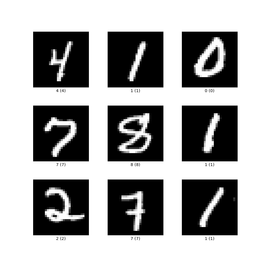
Let’s visualize some test samples.
import matplotlib.pyplot as plt
plt.figure(figsize=(12,10))
for i in range(15):
    plt.subplot(5,5,i+1)
    plt.xticks([])
    plt.yticks([])
    plt.grid(False)
    plt.imshow(test_images[i], cmap='gray')
    plt.xlabel(test_labels[i])
plt.show()
Let’s try to plot a color bar of one image and see the pixel intensity distribution of the image.
plt.figure()
plt.imshow(training_images[0])
plt.colorbar()
plt.grid(False)
plt.show()
The color bar of the above figure shows the values in the number are between 0 and 255.
Dividing by 255 ensures that a number between [0,1] represents every pixel. This process is called the normalization of the image. Normalization will improve performance. Usually, If we use non-normalized data, the neural net will not learn properly.
training_images  = training_images / 255.0
test_images = test_images / 255.0
Building the neural network requires configuring the layers of the model, then compiling the model.
The digit dataset is of size (28,28). You cannot fit a two-dimensional array directly into the dense layer. However, you can transform images from a two-dimensional array (of 28 by 28 pixels) to a one-dimensional array (of 28 * 28 = 784 pixels) using the Flatten().
After the pixels are flattened, the network consists of a sequence of two Dense layers.
- The first Dense layer has 256 units of neurons.
- The second layer returns a logits array. There are ten neurons; therefore, the length of the logit array is ten.
Each neuron or node on the last layer contains a score that indicates the class of the given image.
model = tf.keras.models.Sequential([
    tf.keras.layers.Flatten(input_shape=(28, 28)),
    tf.keras.layers.Dense(256, activation=tf.nn.relu),
    tf.keras.layers.Dense(10, activation=tf.nn.softmax)
])
Compile the model
Before the model is ready for training, it needs a few more settings. These are added during the model’s compile step:
loss —This measures how accurate the model is during training. You want to minimize the loss to direct the model training in the right direction.
optimizer — This is how the model is updated based on the data it sees and its loss function.
metrics — Used to monitor the training and testing steps. The following example uses accuracy, the fraction of the images that are correctly classified.
model.compile(optimizer='adam',
                loss='sparse_categorical_crossentropy',
                metrics=['accuracy'])
Let’s train the model up to ten epochs.
history = model.fit(
    training_images, training_labels, epochs=10
)
Epoch 1/10
1875/1875 [==============================] - 6s 3ms/step - loss: 0.2250 - accuracy: 0.9354
Epoch 2/10
1875/1875 [==============================] - 6s 3ms/step - loss: 0.0933 - accuracy: 0.9721
Epoch 3/10
1875/1875 [==============================] - 5s 3ms/step - loss: 0.0605 - accuracy: 0.9816
Epoch 4/10
1875/1875 [==============================] - 5s 3ms/step - loss: 0.0444 - accuracy: 0.9860
Epoch 5/10
1875/1875 [==============================] - 5s 3ms/step - loss: 0.0325 - accuracy: 0.9899
Epoch 6/10
1875/1875 [==============================] - 6s 3ms/step - loss: 0.0250 - accuracy: 0.9919
Epoch 7/10
1875/1875 [==============================] - 6s 3ms/step - loss: 0.0195 - accuracy: 0.9934
Epoch 8/10
1875/1875 [==============================] - 6s 3ms/step - loss: 0.0165 - accuracy: 0.9948
Epoch 9/10
1875/1875 [==============================] - 5s 3ms/step - loss: 0.0130 - accuracy: 0.9958
Epoch 10/10
1875/1875 [==============================] - 5s 3ms/step - loss: 0.0123 - accuracy: 0.9959
How to stop training if the training accuracy reaches 98%?
In the above case, the epochs are hardcoded. We cannot stop the model training if we reach our desired level of accuracy before the end of the epoch. There is no point to tune the epochs value and retrain the model.
The best approach is to use a callback on the training. Callbacks are used to monitor the evaluation metric on model training. In the following section, we will write our custom callback class that will stop model training if the accuracy reaches 98%.
class customCallback(tf.keras.callbacks.Callback):
    def on_epoch_end(self, epoch, logs={}):
        if (logs.get('accuracy') > 0.98):
            print("\nReached 98% accuracy so cancelling training!")
            self.model.stop_training = True
The class customCallback takes a tf.keras.callbacks.Callback as a parameter. Inside it, we have defined the on_epoch_end() function, which will give us details about the logs for each epoch. We will check the value of logs at the end of each epoch and compare the value with the desired level of accuracy. If we have reached the desired level of accuracy, we can stop training by saying self.model.stop_training = True.
To implement the class customCallbacks, we have to instantiate the object of the class.
Let’s create an object named callbacks.
callbacks = customCallback()
mnist = tf.keras.datasets.mnist
(train_images, train_labels), (test_images, test_labels) = mnist.load_data()
train_images, test_images = train_images / 255.0, test_images / 255.0
model = tf.keras.models.Sequential([
    tf.keras.layers.Flatten(input_shape=(28, 28)),
    tf.keras.layers.Dense(512, activation=tf.nn.relu),
    tf.keras.layers.Dense(10, activation=tf.nn.softmax)
])
model.compile(optimizer='adam',
                loss='sparse_categorical_crossentropy',
                metrics=['accuracy'])
Now we have to pass the callbacks object on callback parameter of model.fit() statement.
history = model.fit(
    train_images, train_labels, epochs=10, callbacks=[callbacks]
)
Epoch 1/10
1875/1875 [==============================] - 10s 5ms/step - loss: 0.1994 - accuracy: 0.9407
Epoch 2/10
1875/1875 [==============================] - 9s 5ms/step - loss: 0.0815 - accuracy: 0.9748
Epoch 3/10
1875/1875 [==============================] - 10s 5ms/step - loss: 0.0530 - accuracy: 0.9834

Reached 98% accuracy so cancelling training!
The model stop training after the third epochs.
Model performance on test data
Let’s see how the model performs on the test dataset:
test_loss, test_acc = model.evaluate(test_images,  test_labels, verbose=2)

print('\nTest accuracy:', test_acc)
313/313 - 1s - loss: 0.0654 - accuracy: 0.9792

Test accuracy: 0.979200005531311
Conclusion
The training and testing accuracy of the model is near similar. Therefore, the model trained is not overfitting.
References
[1] Moroney, L. (2020). Ai and machine learning for coders. “ O’Reilly Media, Inc.”.
[2] https://www.tensorflow.org/tutorials/keras/classification