This project aims to detect and recognize Nepali cash using transfer learning and the InceptionV3 model. The model achieved 93.03% accuracy on both test and validation data. [Last updated: 2023 with more class and dataset]

Nepali Cash Detection and Recognition Using Transfer Learning and InceptionV3

Repo

Dataset

The dataset used in this project consists of images of Nepali cash denominations. The dataset contains seven classes, namely:

• fifty
• five
• fivehundred
• hundred
• ten
• thousand
• twenty

Model

Transfer learning was used to train the model using the InceptionV3 architecture. The model was trained on the dataset for 10 epochs with a batch size of 64. The model achieved an accuracy of 91% on both test and validation data.

Results

The model achieved an accuracy of 95% on training data and 93% (approx) on validation data. Similarly following performance on test data.

• Precision = 93.03%
• Recall = 93.03%
• F1-score = 93.03%

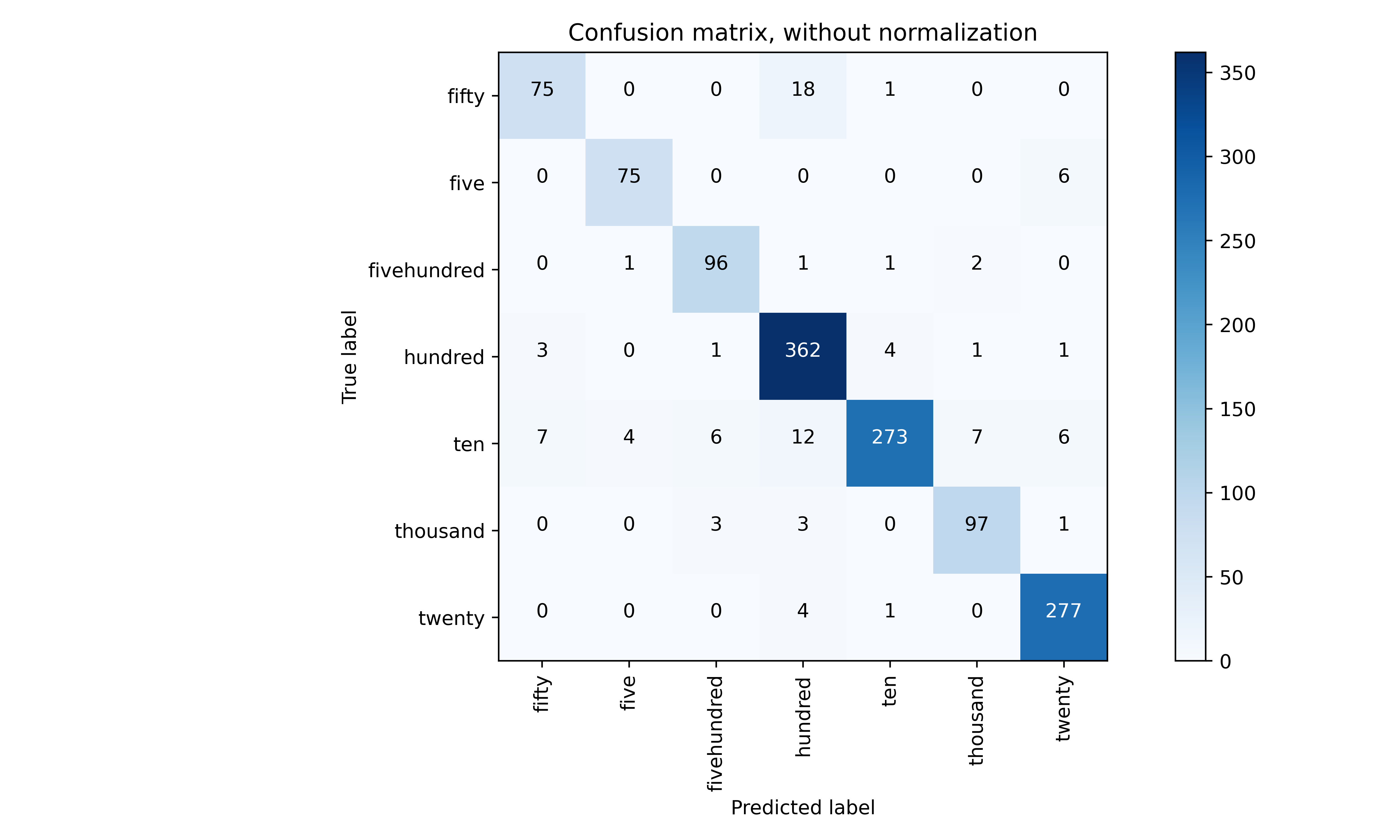
The confusion matrix for the model on test data is shown below:

A confusion matrix is a table that is often used to evaluate the performance of a classification model. The matrix compares the actual class labels of the test data with the predicted labels given by the model.

A confusion matrix typically has rows representing the true labels and columns representing the predicted labels. Each element of the matrix represents the count or number of instances that belong to a particular combination of true and predicted labels.

In the example matrix given above, the true labels are: fifty, five, fivehundred, hundred, ten, thousand, twenty. The predicted labels are the same.

The diagonal of the matrix shows the number of true positives (i.e., correct predictions) for each class, and the off-diagonal elements show the number of false positives (i.e., incorrect predictions) for each class.

For example, the element in the first row and first column represents the number of instances that truly belong to the class ‘fifty’ and were predicted as ‘fifty’ by the model. In this case, the value is 75.

Again we can see that there are 1 instance of ‘hundred’ that were misclassified as ‘fivehundred’ by the model.

By analyzing the confusion matrix, we can evaluate the performance of the model and identify the areas where the model is making mistakes.

For example, in the above matrix, we can see that the model is confusing the classes and has misclassified 6 instances of 10 as 500. We can use this information to improve the model’s performance, for example by increasing the amount of training data or tweaking the model’s hyperparameters.

Training and Validation Accuracy

The above figure shows the model is being trained and evaluated for 17 epochs. The model’s performance is evaluated on a validation dataset after each epoch to check if the model is overfitting or learning general patterns.

Accuracy measures how well the model is able to classify images in the training data, while val_accuracy measures how well the model generalizes to new, unseen data.

Both metrics should ideally increase over time, but if accuracy is significantly higher than val_accuracy, the model may be overfitting, and if val_accuracy is consistently higher than accuracy, the model may be underfitting. The training accuracy measures how well the model is learning the patterns in the training data, while the validation accuracy measures how well the model is generalizing to new data.

In this example, we can see that the model starts with a training accuracy of 0.68 and a validation accuracy of 0.87 in the first epoch. This means that the model is performing better on the validation dataset than the train dataset, indicating that it may be underfitting.

However, as the number of epochs increases, we can see that the validation accuracy also increases, reaching a maximum of 0.92 in the thirteen epoch. This suggests that the model is learning more general patterns that can be applied to new data.

The training and validation accuracy are increasing over time, which indicates that the model is learning features and generalizing well on unseen data. The use of EarlyStopping, ModelCheckpoint, and Dropout layers helps to avoid overfitting.

The training accuracy starts at 68.43% and increases to 96.35% by the end of the training. Similarly, the validation accuracy starts at 87.14% and increases to 91.19% by the end of the training. This indicates that the model is performing well on both the training and validation datasets.

The use of ModelCheckpoint ensures that the best performing model is saved during training, which can be used for later testing or deployment. The use of EarlyStopping ensures that the training process stops if the validation accuracy does not improve for a certain number of epochs, which helps to prevent overfitting.

Overall, the training process seems to be well-optimized and the model is performing well on the dataset.

Training and validation loss

In the context of a machine learning model, the training and validation loss are measures of how well the model is performing during the training and validation phases, respectively.

The loss function is a measure of how well the model is able to predict the correct output. During training, the model is adjusted to minimize this loss. A low training loss indicates that the model is fitting the training data well, whereas a high training loss indicates that the model is not fitting the data well.

Validation loss is the loss computed on a set of data that is not used for training, and it is used to assess how well the model is generalizing to new data. If the validation loss is low, it indicates that the model is performing well on unseen data. If the validation loss is much higher than the training loss, it may indicate that the model is overfitting the training data and is not generalizing well.

In the above figure, The loss function also shows a decreasing trend for both the training and validation sets, which indicates that the model is learning to minimize the error between the predicted and actual values.

Conclusion

In conclusion, this project has demonstrated the effectiveness of transfer learning and the InceptionV3 model for detecting and recognizing Nepali cash denominations with an accuracy of 91%.

Streamlit web application

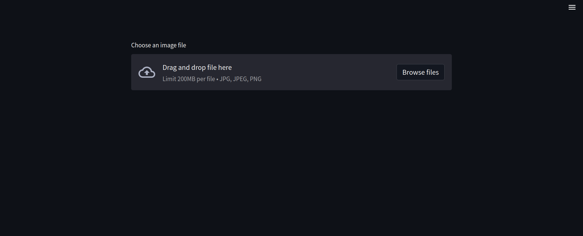
Repository: Nepali Cash Recogniton and Detection To run the application, you need to have Streamlit installed on your computer. If you don’t have Streamlit installed, you can install it by running the following command in your terminal or command prompt:

pip install streamlit

Once Streamlit is installed, navigate to the directory where your main.py file is located using your terminal or command prompt. Then, run the command:

streamlit run main.py

This should start the Streamlit server and open the web application in a new tab in your default web browser.

Now Upload the Images inside image-data-inference

Another Example

Note

The Streamlit application also has the capability to audibly identify the type of banknote.

How overfitting is handled?

Overfitting is a common problem in image classification tasks, where the model learns to fit the training data too well, resulting in poor generalization on unseen data. To avoid overfitting, there are several techniques are used:

• Data Augmentation: This involves generating new training data by applying transformations such as rotation, zoom, shift, etc. to the original images. This increases the diversity of the training data and helps the model learn more robust features.

• Dropout: This is a regularization technique that randomly drops out a fraction of neurons in the network during training, which helps prevent the network from relying too heavily on any single feature.

• Early Stopping: This involves monitoring the validation loss during training and stopping the training process when the validation loss starts to increase. This prevents the model from overfitting by stopping training before it starts to memorize the training data.

• Transfer Learning: This involves using a pre-trained model as a starting point and fine-tuning it on the new dataset. This can be an effective way to avoid overfitting, as the pre-trained model has already learned general features that can be useful for the new task.